Kernel Logistic Regression

This is my implementation for the Kernel Logistic Regression using linear empirical risk minimization to learn nonlinear decision boundaries.
Author

Kent Canonigo

Published

March 9, 2023

Kernel Logistic Regression Implementation

Here is the link to my source code: Kernel Logistic Regression

Empirical Risk Loss

In the Gradient Descent blog post, we computed the empirical risk equation: \[L(w) = \frac{1}{n}\sum_{i=1}^{n} \ell({\langle w, x_{i} \rangle, y_{i})}\]

where the logistic loss was: \[ \ell({\hat{y}, y}) = -y * log(\sigma(\hat{y})) - (1-y)* log(1-\sigma(\hat{y})) \]

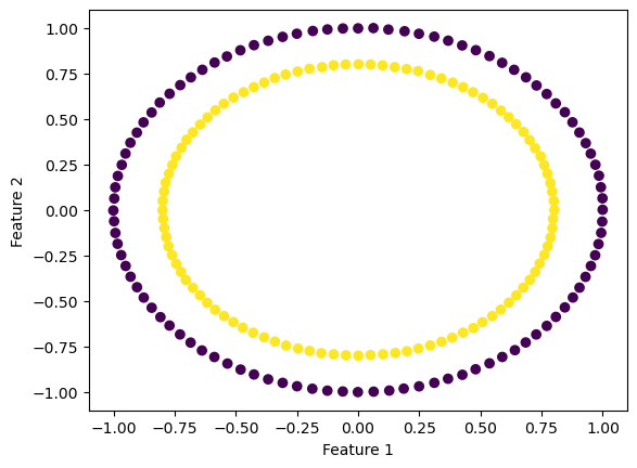
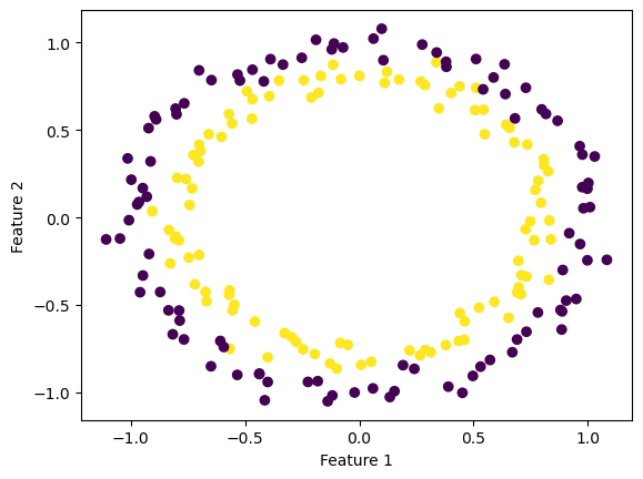
For the kernel logistic regression, by using the kernel trick, we are able to modify our feature matrix \(X\) to be of infinite-dimensional. This means that by transforming our feature matrix X to a kernel matrix, we are able to extend the binary classification of logistic regression for nonlinear features.

Now, the empirical risk for the kernel logistic regression looks like:

\[L(w) = \frac{1}{n}\sum_{i=1}^{n} \ell({\langle v, \kappa({x_{i}}) \rangle, y_{i})}\]

where \(\kappa({x_{i}})\) represents the modified feature vector with row dimension \(\in{R^n}\).

To translate the new empirical risk for the kernel logistic regression into code, I modified my empirical_risk method to take in additional parameters \(km\) and \(w\); \(km\) represents the kernel matrix, and \(w\) represents the weight vector to be optimized. Additionally, I modified my logistic loss method such that it now takes in a pre-computed y_hat as a parameter (originally, the method had taken in a y_hat using the predict method).

We use this loss method to compute the empirical risk by using the inner product between \(km\) and our weight vector \(w\) as our y_hat. Finally, we can take the mean of the loss of the inner product and the true label y to generate our overall empirical risk loss.

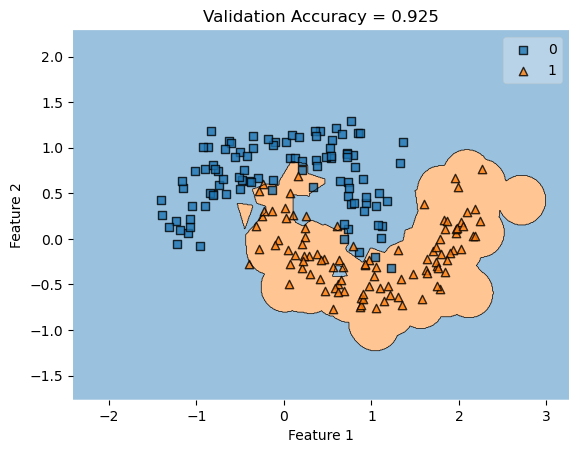
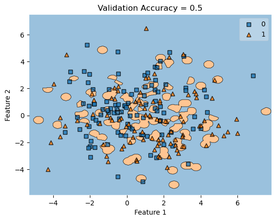
In my fit method, one challenge I faced was the structure of the optimized \(w\) weight vector. In this implementation, I had used the function scipy.optimize.minimize() to optimize my \(w\); the optimized \(w\), however, continuously generated a vector of positive values. This would cause an error in my experiments as the plot_decision_regions function will not be able to plot the trained model’s score.

To fix this problem, after initializing some initial vector \(w_0\) of dimension \(X.shape[0]\), I subtracted \(w_0\) by \(0.5\) to generate both negative and positive values in the optimized \(w\) weight vector.

Experiments

Basic Check

To test the correctness of my kernel logistic regression implementation, I can fit the model to some non-linear data to consistently get an accuracy of the training data at or above \(90\)%. However, there are times when the accuracy is significantly below the \(90\)% threshold; the function scipy.optimize.minimize() is unable to detect the gradient of the empirical risk. Thus at each iteration, the function is estimating the gradient until it reaches some “optimized” weight vector \(w\).

from kernel import KernelLogisticRegression 
from sklearn.metrics.pairwise import rbf_kernel
from sklearn.datasets import make_moons, make_circles
import numpy as np 

np.random.seed(12)

X, y = make_moons(200, shuffle = True, noise = 0.222)
KLR = KernelLogisticRegression(rbf_kernel, gamma = .1)
KLR.fit(X, y)
print("This is the model's accuracy: ", KLR.score(X, y))
This is the model's accuracy:  0.91

Choosing gamma

In the experiment above, I’ve tested my implementation of kernel logistic regression choosing a small gamma value of \(0.1\). However, what if I decide to use a gamma value significantly larger than \(0.1\)? For this experiment, let’s compare trained models with a small gamma. Let the larger gamma value be \(10000\), and let’s see what happens.

Shown below is some randomly generated nonlinear data of features. For this experiment, I’ve fixed the noise of the data to be \(0.222\).

from sklearn.datasets import make_moons, make_circles
from matplotlib import pyplot as plt
import numpy as np
np.random.seed(12)

np.seterr(all="ignore")


X, y = make_moons(200, shuffle = True, noise = 0.222)
plt.scatter(X[:,0], X[:,1], c = y)
labels = plt.gca().set(xlabel = "Feature 1", ylabel = "Feature 2")

from mlxtend.plotting import plot_decision_regions

np.random.seed(12)

KLR = KernelLogisticRegression(rbf_kernel, gamma = .1)
KLR.fit(X, y)
plot_decision_regions(X, y, clf = KLR)
t = title = plt.gca().set(title = f"Training Accuracy = {KLR.score(X, y)}",
                      xlabel = "Feature 1", 
                      ylabel = "Feature 2")

Then, we can use this trained model on some new unseen data to test its validation accuracy.

X, y = make_moons(200, shuffle = True, noise = 0.222)
plot_decision_regions(X, y, clf = KLR)
title = plt.gca().set(title = f"Validation Accuracy = {KLR.score(X, y)}",
                      xlabel = "Feature 1", 
                      ylabel = "Feature 2")

As shown above, the validation accuracy for the trained model with a gamma value of \(0.1\) shows similar performance to the testing accuracy above the \(90\)% accuracy threshold.

Next, we can do the same for a model with a gamma value of \(10000\). In this case, we can expect that the testing accuracy to be \(1.0\) because the model will overfit. If the testing accuracy is \(1.0\), how will the validation accuracy hold on some unseen test data?

np.random.seed(15)

X, y = make_moons(200, shuffle = True, noise = 0.222)
KLR = KernelLogisticRegression(rbf_kernel, gamma = 10000)
KLR.fit(X, y)
plot_decision_regions(X, y, clf = KLR)
t = title = plt.gca().set(title = f"Training Accuracy = {KLR.score(X, y)}",
                      xlabel = "Feature 1", 
                      ylabel = "Feature 2")

X, y = make_moons(200, shuffle = True, noise = 0.222)
plot_decision_regions(X, y, clf = KLR)
title = plt.gca().set(title = f"Validation Accuracy = {KLR.score(X, y)}",
                      xlabel = "Feature 1", 
                      ylabel = "Feature 2")

Even though our training accuracy is \(1.0\), our validation accuracy decreases and does not fully reach \(1.0\) accuracy, but the validation accuracy is still above the \(90\)% threshold. So, does that mean that this overfit model is still good enough? In truth, we should expect that the validation accuracy to be significantly lesser than the training accuracy. In the next experiment, we’ll vary the noise such that by observation, we can conclude that the validation accuracy will be significantly worse in generalization for an overfit model.

Varying Noise

In this experiment, we will repeat the previous experiments with varied noise. How does the choices of noise affect our initial data?

np.random.seed(15)

X, y = make_moons(200, shuffle = True, noise = 0.001)
plt.scatter(X[:,0], X[:,1], c = y)
labels = plt.gca().set(xlabel = "Feature 1", ylabel = "Feature 2")

Shown above, I’ve fixed the noise to be \(0.001\). By observation, choosing some very small noise makes similar feature points closer to each other.

np.random.seed(16)

X, y = make_moons(200, shuffle = True, noise = 0.1)
plt.scatter(X[:,0], X[:,1], c = y)
labels = plt.gca().set(xlabel = "Feature 1", ylabel = "Feature 2")

np.random.seed(17)

X, y = make_moons(200, shuffle = True, noise = 1)
plt.scatter(X[:,0], X[:,1], c = y)
labels = plt.gca().set(xlabel = "Feature 1", ylabel = "Feature 2")

In the two plots above, I’ve increased the noise to be \(0.1\) and \(1\). It is observed for the crescent-like data to be increasingly nonlinear and dispersed throughout the region. Now, we can experiment how varied noise level affects the training and validation accuracy using kernel logistic regression.

In the previous experiment, I’ve fixed noise to be a relatively small value of \(0.222\). Let’s choose a lesser and greater noise value of \(0.05\) and \(1\) and observe what happens to the decision regions when plotted on the trained models. We’ll perform each model twice to record its performance for a smaller and larger noise level with a gamma level of \(0.1\).

Small Noise

np.random.seed(18)

X, y = make_moons(200, shuffle = True, noise = 0.05)
KLR = KernelLogisticRegression(rbf_kernel, gamma = 0.1)
KLR.fit(X, y)
plot_decision_regions(X, y, clf = KLR)
t = title = plt.gca().set(title = f"Training Accuracy = {KLR.score(X, y)}",
                      xlabel = "Feature 1", 
                      ylabel = "Feature 2")

np.random.seed(19)
X, y = make_moons(200, shuffle = True, noise = 0.05)
plot_decision_regions(X, y, clf = KLR)
t = title = plt.gca().set(title = f"Validation Accuracy = {KLR.score(X, y)}",
                      xlabel = "Feature 1", 
                      ylabel = "Feature 2")

For a fitted model whose gamma and noise levels are small, both training and validation accuracy are highly accurate and shows similar performance above the \(90\)% accuracy threshold.

Large Noise

np.random.seed(20)

X, y = make_moons(200, shuffle = True, noise = 1)
KLR = KernelLogisticRegression(rbf_kernel, gamma = 0.1)
KLR.fit(X, y)
plot_decision_regions(X, y, clf = KLR)
t = title = plt.gca().set(title = f"Training Accuracy = {KLR.score(X, y)}",
                      xlabel = "Feature 1", 
                      ylabel = "Feature 2")

np.random.seed(21) 

X, y = make_moons(200, shuffle = True, noise = 1)
plot_decision_regions(X, y, clf = KLR)
t = title = plt.gca().set(title = f"Validation Accuracy = {KLR.score(X, y)}",
                      xlabel = "Feature 1", 
                      ylabel = "Feature 2")

However, for a model with a small gamma and a data with large noise, the model can only do so much to classify the heavily dispersed and nonlinear data. The training accuracy no longer goes at or above the \(90\)% threshold we’ve seen before, but considering the large noise level, a small gamma still generates moderate accuracy in classifying the features.

For the gamma experiment, we concluded that a smaller gamma value will produce a higher validation accuracy. However, our choice of the gamma actually depends on the choice of noise. A smaller noise will generate a higher validation accuracy than choosing a data with large noise.

Large Gamma and Noise

In the gammaexperiment, we tested an overfit model for some data of small noise and a gamma value of \(10000\) and observed that its validation accuracy was still above the \(90\)% threshold. In this experiment, I will display the results for an overfit model of data with large noise; I’ve chosen the same gamma value and set the data noise to be \(2\).

np.random.seed(22)

X, y = make_moons(200, shuffle = True, noise = 2)
KLR = KernelLogisticRegression(rbf_kernel, gamma = 10000)
KLR.fit(X, y)
plot_decision_regions(X, y, clf = KLR)
t = title = plt.gca().set(title = f"Training Accuracy = {KLR.score(X, y)}",
                      xlabel = "Feature 1", 
                      ylabel = "Feature 2")

np.random.seed(23)

X, y = make_moons(200, shuffle = True, noise = 2)
plot_decision_regions(X, y, clf = KLR)
t = title = plt.gca().set(title = f"Validation Accuracy = {KLR.score(X, y)}",
                      xlabel = "Feature 1", 
                      ylabel = "Feature 2")

Shown above, we’ve plotted the decision regions for an overfit model with a gamma value of \(10000\) for a data with noise \(2\). Though the training accuracy was \(1.0\), generalizing the model on unseen test data generated a validation accuracy of \(0.5\) which is significantly worse; the model successfully classifies and predicts for unseen test data \(50\)% of the time. In contrast to the previous overfit model experiment, we can conclude that choosing a large noise will significantly decrease the validation accuracy below the \(90\)% threshold.

Other Geometries

In the previous experiments, we’ve generated a moon shaped data. However, will our trained model using kernel logistic regression generate high validation accuracy for a circle-shaped data?

In this experiment, I will generate concentric circles instead of crescents using the make_circles function. Shown below are several examples of circle-shaped data with varying noise.

np.random.seed(24)
# Small noise
X, y = make_circles(n_samples= 200, noise=0.001, shuffle = True)
plt.scatter(X[:,0], X[:,1], c = y)
labels = plt.gca().set(xlabel = "Feature 1", ylabel = "Feature 2")

np.random.seed(25)
# Medium noise
X, y = make_circles(n_samples= 200, noise=0.05, shuffle = True)
plt.scatter(X[:,0], X[:,1], c = y)
labels = plt.gca().set(xlabel = "Feature 1", ylabel = "Feature 2")

np.random.seed(26)
# Large noise
X, y = make_circles(n_samples= 200, noise=1, shuffle = True)
plt.scatter(X[:,0], X[:,1], c = y)
labels = plt.gca().set(xlabel = "Feature 1", ylabel = "Feature 2")

For this experiment, we’ll generate a circle-shaped data with small noise and fit our model with small gamma to generate both high testing and validation accuracy. For this experiment, I’ve chosen a noise of \(0.05\).

np.random.seed(27)

X, y = make_circles(n_samples= 200, noise=0.05, shuffle = True)
KLR = KernelLogisticRegression(rbf_kernel, gamma = 0.1)
KLR.fit(X, y)
plot_decision_regions(X, y, clf = KLR)
t = title = plt.gca().set(title = f"Training Accuracy = {KLR.score(X, y)}",
                      xlabel = "Feature 1", 
                      ylabel = "Feature 2")

# Test our trained model on unseen test datta
X, y = make_circles(n_samples= 200, noise=0.05, shuffle = True)
plot_decision_regions(X, y, clf = KLR)
title = plt.gca().set(title = f"Validation Accuracy = {KLR.score(X, y)}",
                      xlabel = "Feature 1", 
                      ylabel = "Feature 2")

Shown above, we observed that by choosing some small gamma and noise for a circle-shaped data, our trained model generated both high training and validation accuracy above the \(90\)% threshold. Thus, this is a pretty successful classifier.